How to: Create a Heatmap Raster in PostGIS and Render in GeoServer

In this post, we are going to explore a little of the the raster processing capabilities of the powerful PostgreSQL extension – PostGIS.

We will be doing the following steps in this tutorial:

1. Create a PostGIS raster and populate it’s pixel values.
2. Export the raster data as a file in TIFF format
3. Convert the TIFF to GeoTIFF or World Image format using GDAL
4. Create a store in GeoServer using the GeoTIFF or Word Image
5. Create style(SLD) for the raster and render/display the layer in real map

A short introduction to the Raster World

WKT Raster is a raster format developed by PostGIS which support multi-band, georefernce and overlapping tiles. There are also a number of functions available to manipulate and perform magnificent analysis on the raster data. The WKT Raster is so integrated with the PostGIS geometry data type that we can apply geometry function to raster and intersect it with vector data to perform various operations.

INSERT INTO raster_table(rid,rast)
VALUES(1, ST_MakeEmptyRaster( 100, 100, 3087924.140142075, -2973362.7697100244, 5, 5, 0, 0, 900913) );

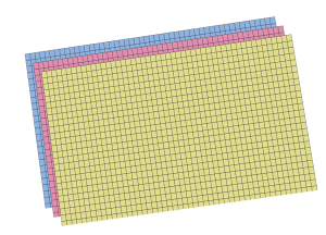
The above query will generate an empty raster with a width and height of 100 pixels and upper left x and y coordinates (3087924.140142075, -2973362.7697100244). Each pixel is having a width and height of 5 geographic unit according to the projection 900913. So this raster will sit somewhere in South Africa, spanning a 500m x 500m rectangular area!

As shown in the image, our raster is divided into 100 rows and columns, wherein each cell have an area of 5m x 5m.

Now, that we have an empty raster in hand, next, we have to add bands to our raster. You can think of bands like a canvas where in each cell you can fill numeric values. You can have multiple bands in the same raster so that the same cell can have different numeric values (pixel values) in each band.

To add a band to our raster we can make use of the ST_AddBand function.

UPDATE raster_table
SET rast = ST_AddBand(rast, 1, '32BF', 0)
WHERE rid = 1;

This command will add a new band to our raster with band index, 1 and PixelType, 32 bit float. Setting pixelType 32BF let us store any 32 bit floating point number to any pixel/cell of our raster. There are also many other PixelTypes available for use.

Populate Pixel Values

To set values to a single pixel of  the rater we can use the ST_SetValue function. For instance, we can set a value to the pixel at the center point of our raster as follows:

UPDATE raster_table
SET rast = ST_SetValue(rast, 1, ST_GeomFromText('POINT(3088174.140142075 -2973112.769710024)',900913) , 300.25)
WHERE rid = 1;

Note that, since we have passed the geometric point as the input, the value will be set to the pixel which contains that point.

Setting values with ST_SetValue is inefficient because it can set only one value at a time. There are another variant of this function – ST_SetValues, which can set multiple value at a time:

UPDATE raster_table
SET rast = ST_SetValues(rast, 1, ARRAY[ROW(ST_GeomFromText('POINT(3088174.140142075 -2973112.769710024)',900913), 300.25),
ROW(ST_GeomFromText('POINT(3088184.140142458 -2973082.769710025)',900913), 200.454)]::geomval[])
WHERE rid = 1;

The ST_SetValues function is only available for PostGIS 2.1 and later. For older versions the only option is to use ST_SetValue.

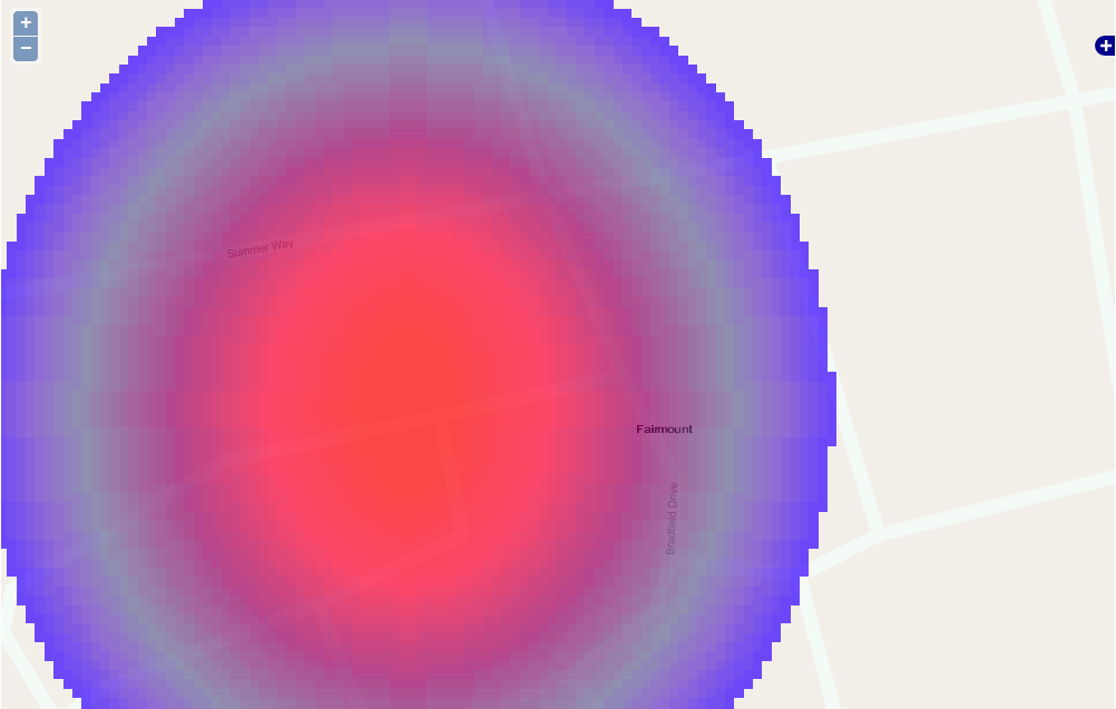
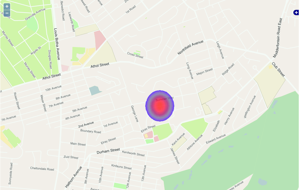
Now, let’s write a function which set values in an elliptical path, starting from the center point, heading towards the edges of our raster. Each path will have a set of points/pixels having a common pixel value.  This function is the base to generate the beautiful heat map seen in the introductory section.

CREATE OR REPLACE FUNCTION create_elliptical_raster()
RETURNS character varying AS
$BODY$
DECLARE
dist double precision = 0.5;
point_x double precision;
point_y double precision;
value double precision = 600;
query_part varchar = '';
query varchar = '';
i double precision = 0;
BEGIN
WHILE(dist + 20 <= 250) LOOP

WHILE i <= 360 LOOP
point_x = 3088174.140142075 + (dist * cos(i));
point_y = -2973112.769710024 + ((dist + 20) * sin(i));
value = value - 10;
i = i + .02;
query_part = query_part || ',' || 'ROW(st_setsrid(''POINT('||point_x||' '||point_y||')''::geometry, 900913), '||value||')';
END LOOP;

query_part = substring(query_part from 2 for (length(query_part)-1));
query = 'UPDATE raster_table SET rast = ST_SetValues(rast, 1, ARRAY['|| query_part ||']::geomval[]) WHERE rid = 1';
EXECUTE query;
query_part = '';
query = '';
dist = dist + 5;
i = 0;
END LOOP;

RETURN 'SUCCESS';
END;
$BODY$
LANGUAGE plpgsql VOLATILE
COST 100;

To see a preview of our raster we use the open source GIS application – OpenJump.

Export PostGIS Raster as TIFF File

Unfortunately GeoServer have no provision to load a raster directly from database. So, we have to export our raster in TIFF format, which GeoServer can recognize.

To export raster as TIFF, first, we find the oid of the raters’ lob(large object) using the query below:

SELECT oid, lowrite(lo_open(oid, 131072), png) As num_bytes
FROM
( VALUES (lo_create(0),
ST_Astiff( (SELECT rast FROM raster_table WHERE rid = 1) )
) ) As v(oid,png);

Secondly, we use the PostgreSQL \lo_export command to output our raster as a tiff file:

\lo_export 147303 '/tmp/heatmapellipsegeo.tiff'

Convert TIFF to GeoTIFF or WorldImage Format

GeoTIFF and WorldImage are two raster file formats supported by GeoServer. To convert our raster to these formats we may use the GDAL library.

 To install GDAL library and tools in linux/ubuntu use: apt-get install gdal-bin

 The GeoTIFF format will contain additional headers which defines the geolocation and projection information. To convert our TIFF to GeoTIFF use the gdal_translate utility as follows:

gdal_translate /tmp/heatmapellipse.tiff -of GTiff -a_srs 'PROJCS[AUTHORITY["EPSG","900913"]]' -a_nodata 0 /tmp/heatmapellipsegeo.tiff

 Though we have converted the raster to GeoTIFF with 900913 projection, geoserver do have some problem in recognizing this particular projection’s WKT. This problem is still open, but is not existing for any other projections. A discussion on this issue can be found here.

Now, let’s see how we can convert our raster file to WorldImage format. A WorldImage is composed of two files: one TIFF and a TFW file. TFW is a plain text file having the geoinformations. We, again, use gdal_translate to generate a TFW out of our raster TIFF:

gdal_translate -co "TFW=YES" heatmapellipse.tiff heatmapellipse1.tiff

This will generate two new files: heatmapellipse1.tiff and heatmapellipse1.tfw

Create GeoServer Raster Store / Data Source

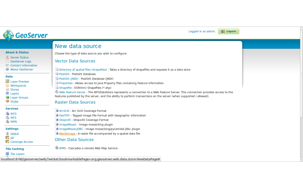
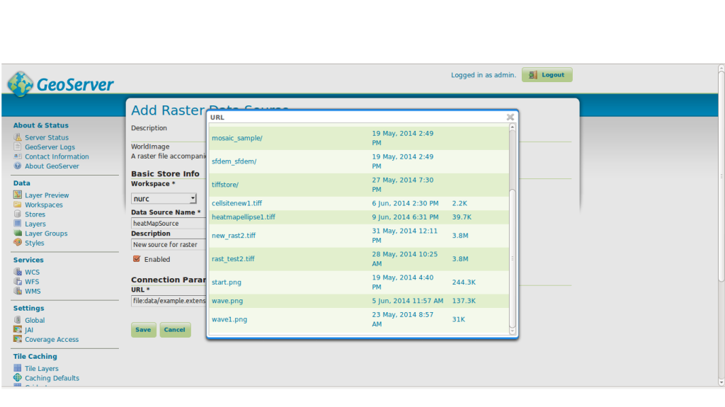
In this step, we will create a Store using our WorldImage raster file. Login to your GeoServer control panel and navigate to ‘Stores’.

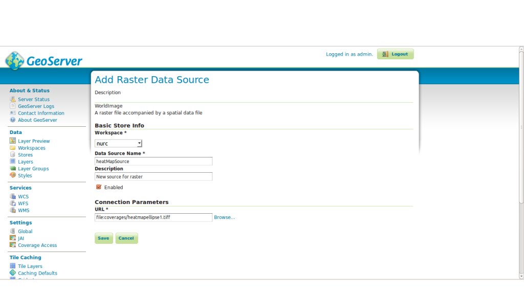
As shown in the above image we will choose to create a WordImage Raster Data Source and proceed to import the WorldImage file we created:

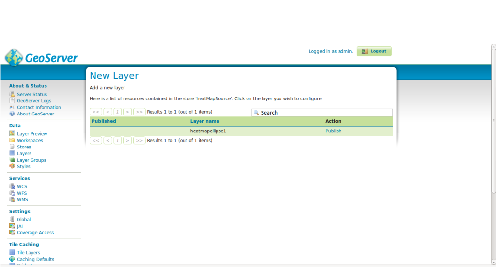
Saving this data source will proceed us to the window showing the layers under the store:

On clicking Publish, we will get the window where we can change the parameters if needed:

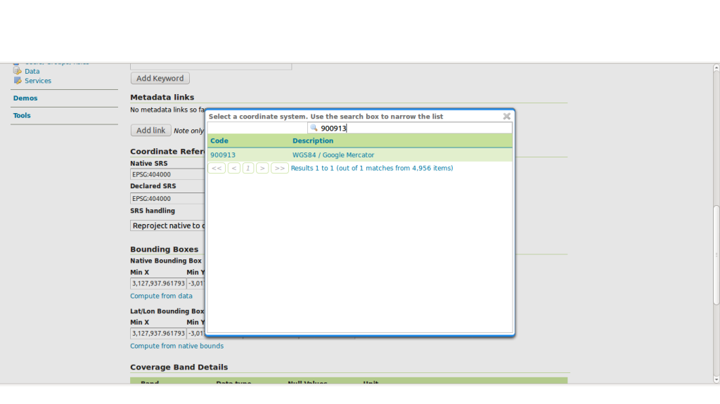
Here, we need to change the declared projection to 900913, since our raster is created with the same. After selecting the 900913 projection and refreshing the declared bound box, switch to the Publish tab and select a style and Save. This step assumes that you have created a raster style using, in prior, which can be like the below SLD:

<?xml version="1.0" encoding="ISO-8859-1"?>
<StyledLayerDescriptor version="1.0.0"
xsi:schemaLocation="<a href="http://www.opengis.net/sld">http://www.opengis.net/sld</a> StyledLayerDescriptor.xsd"
xmlns="<a href="http://www.opengis.net/sld">http://www.opengis.net/sld</a>"
xmlns:ogc="<a href="http://www.opengis.net/ogc">http://www.opengis.net/ogc</a>"
xmlns:xlink="<a href="http://www.w3.org/1999/xlink">http://www.w3.org/1999/xlink</a>"
xmlns:xsi="<a href="http://www.w3.org/2001/XMLSchema-instance">http://www.w3.org/2001/XMLSchema-instance</a>">
<!-- a Named Layer is the basic building block of an SLD document -->
<NamedLayer>
<Name>default_polygon</Name>
<UserStyle>
<!-- Styles can have names, titles and abstracts -->
<Title>Default Polygon</Title>
<Abstract>A sample style that draws a polygon</Abstract>
<!-- FeatureTypeStyles describe how to render different features -->
<!-- A FeatureTypeStyle for rendering polygons -->
<FeatureTypeStyle><Rule><RasterSymbolizer><Opacity>1.0</Opacity>
<ContrastEnhancement>
<GammaValue>1</GammaValue>
</ContrastEnhancement>
<OverlapBehavior>
<AVERAGE />
</OverlapBehavior>
<ColorMap>
<ColorMapEntry color="#FFFFFF" quantity="0" opacity = "0.0"/>
<ColorMapEntry color="#3300FF" quantity="150"/>
<ColorMapEntry color="#6633CC" quantity="200"/>
<ColorMapEntry color="#666699" quantity="250"/>
<ColorMapEntry color="#990066" quantity="350"/>
<ColorMapEntry color="#FF0033" quantity="450"/>
<ColorMapEntry color="#FF0000" quantity="550"/>
</ColorMap></RasterSymbolizer></Rule></FeatureTypeStyle>
</UserStyle>
</NamedLayer>
</StyledLayerDescriptor>

Now, we all set ready to show our raster in the map. Add this WMS layer we created to your map as you like:

var jpl_wms = new OpenLayers.Layer.WMS(
 "Global Imagery",
 "<a href="http://localhost:8180/geoserver/nurc/wms">http://localhost:8180/geoserver/nurc/wms</a>",
 {layers: "heatmapellipse1",transparent:true},
 {displayProjection: new OpenLayers.Projection('EPSG:4326')}
 );
jpl_wms.opacity=0.7;

 

Do More with Rasters!

So far we have seen how to create a raster from scratch and render it in map. The raster we created is for illustration purpose only and is almost meaningless. Instead, we could create rasters visualizing meaningful data such as elevation, signal strength of antennas etc. Go ahead & start designing your raster! Feel free to ask any questions here.

—————————————————–

Co-written by Vipin Raj & Anand Govind CG